Pivot Tables are one of Excel's most powerful features. A Pivot Table allows you to extract the significance from a large, detailed data set.
Creating a PivotTable
- Click any cell within the data set to be analyzed
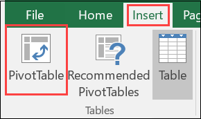
- Navigate to the Insert tab on the Ribbon
- In the Tables group, click the PivotTable button
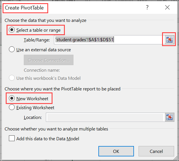
- A Create PivotTable dialog box will appear
*NOTE: When creating a PivotTable without previously creating a Table, make sure your data has column headings or table headers, and that there are no blank rows in the data set
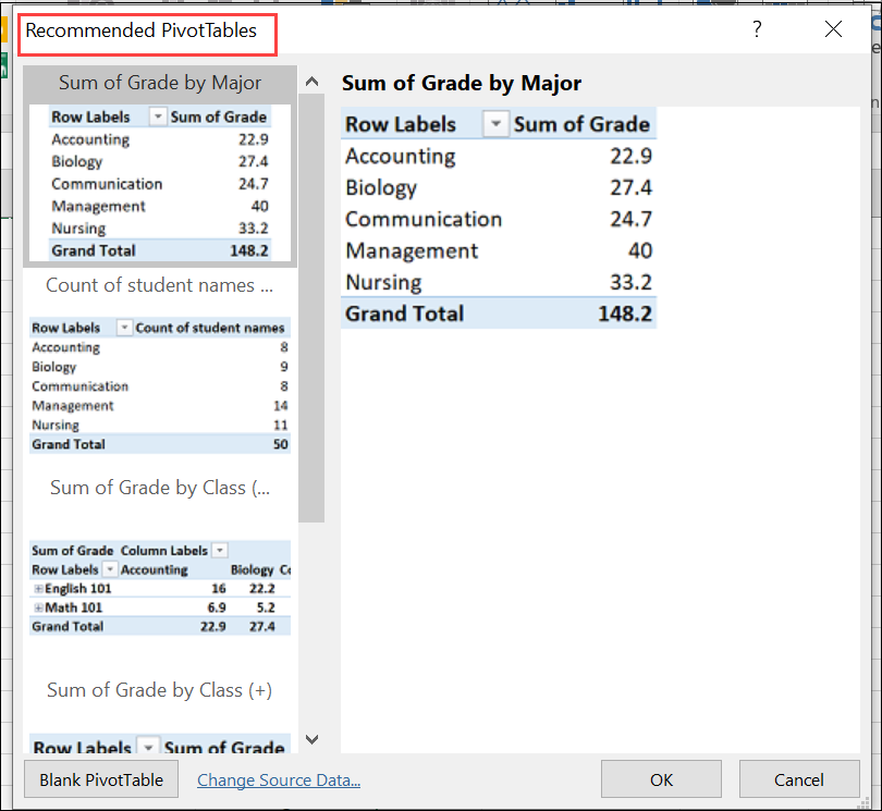
For recommendations on analyzing your data with a PivotTable, click the Recommended PivotTables button and select the desired PivotTable option
- Excel automatically selects the data range for your PivotTable; to change it, click the box at the right of the Table/Range field and select the desired data range
- The default location for the PivotTable is a New Worksheet; to change, click the appropriate button and indicate the desired location
Designing the PivotTable
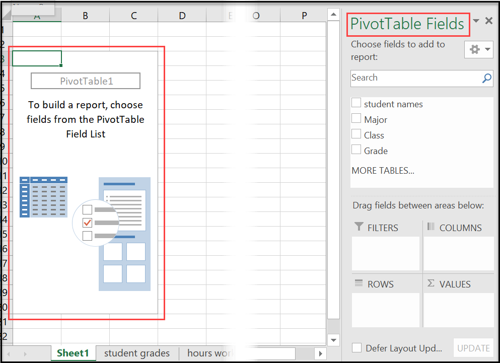
After the PivotTable is created, the PivotTable Fields pane is displayed so fields may be arranged.
- A Field Section for dragging fields to and from the layout section defaults to the top
- A Layout Section for rearranging and repositioning fields defaults to the bottom
- Values - contains the fields that determine which data is presented in the cells of the PivotTable –the values are summarized in its last column
- Row Labels –contains the fields that determine the arrangement of data shown in the rows of the PivotTable
- Column Labels –contains the fields that determine the arrangement of data shown in the columns of the PivotTable.
- Report Filter - contains the fields that act as the filters for the report.
- Under Choose fields to add to the report select and drag the fields to the desired section
The PivotTable Fields List disappears when you click outside of the PivotTable
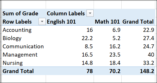
Analyze & Design
Use the PivotTable Tools contextual tab on the Ribbon to Analyze and Design your PivotTable

Change Summary Calculation
By default, Excel summarizes your data by either summing or counting the items. To change the type of calculation you want to use:
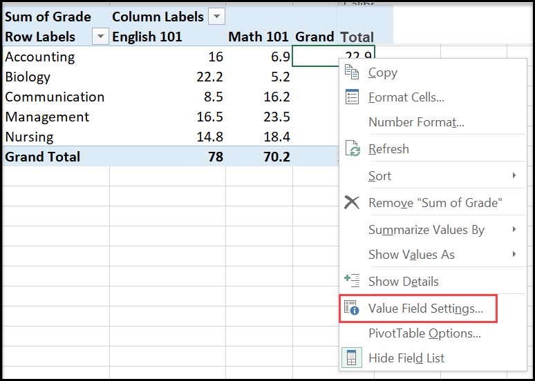
- Click any cell in the Total column
- Right click and select Value Field Settings
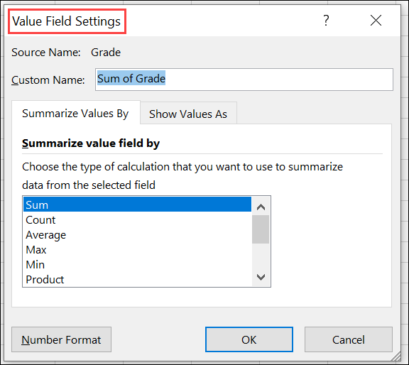
- In the Value Field Settings dialog box, choose the type of calculation you want to use
*NOTE: Format numbers as desired by selecting the Number Format button
Creating a PivotChart
- From an existing PivotTable
- Click anywhere in the PivotTable and go to PivotTable Tools contextual tab
- Under the Analyze tab, in the Tools group, select PivotChart and the type of chart desired
- The Column Labels become the Legend Fields
- Use the PivotChart Tools contextual tab or the Chart Elements tool to format your PivotChart


- From scratch (without an existing PivotTable)
- Click anywhere in your data set
- Navigate to the Insert tab, Charts group
- Click the PivotChart drop down, select PivotChart, or PivotChart & PivotTable to create both simultaneously
- Indicate your data range and where you would like the PivotChart to appear, just as you did for a PivotTable

It is important to “refresh” a PivotTable to update changes to the original data that may have taken place since the creation of the Table.